The Transformer Architecture Explained

A deep dive into the Attention is All You Need paper

The Transformer architecture forms the basis of all large language models (LLMs) like ChatGPT, Llama, Gemini etc.
This architecture has enabled models to generate, reason and manipulate human language at unprecedented scales.
Understanding the Transformer is key to understanding how LLMS work.
Let us dive deep into the original Transformer paper: Attention Is All You Need

The Transformer Architecture

The architecture is divided into 2 parts:

1. Encoder

2. Decoder

Encoder:

The Encoder is tasked with creating a contextualized summary of the input sequences.
An example input sequence is:
‘Messi is the greatest of all time’. Input sequences are the data you feed the model.
Let us see what exactly happens inside the encoder.

Embeddings

We start off by turning our input sequence into embeddings.

An embedding is a learned numerical representation of a word or a token.
So instead of using words themselves, we convert the tokens into a learned numerical representation where similar words have similar values.
We assign embeddings to every unique token in the entire training corpus.
These embeddings are then trained using weights so that they learn similarities between words.

For example, the word ‘good’ and ‘decent’ would have similar values and so will the words ‘good’ and ‘bad’. (even though these words are antonyms, they might be used in the same contexts a lot).

An example of how a sentence is turned into embeddings

Embeddings are trained along with the entire transformer.
Embeddings of each token are stored in a matrix of size [VxD] , where V is the vocabulary size and D is the embedding dimension. Each token ID corresponds to one row in this matrix. During training, the loss gradients update the embeddings alongside all other weights, refining them to capture semantic and syntactic patterns.

Initially, we assign random embeddings to each token which get trained to represent each token better and better with each iteration. They get updated during backpropagation based on the loss function used.

\( W_e \;\leftarrow\; W_e \;-\; \eta \, \frac{\partial \mathcal{L}}{\partial W_e} \)

\(\begin{aligned} \text{where:} \quad & W_e &&= \text{embedding matrix (trainable parameters)} \\ & \eta &&= \text{learning rate} \\ & \mathcal{L} &&= \text{loss function (e.g., cross-entropy)} \\ & \frac{\partial \mathcal{L}}{\partial W_e} &&= \text{gradient of the loss w.r.t. embeddings} \end{aligned}\)

Positional Encoding

Now that we have captured the semantic meaning of each word into numbers, we now use positional encodings for every token in the corpus because transformers have no inherent notion of sequence order.
Positional encodings work the same way as embeddings do, but instead of capturing the semantic meaning, they capture the positioning of tokens.

Words can’t just appear in any position, so we teach the model to remember the fact that certain words appear in certain positions.
For example, the word ‘I’ can appear at the beginning of the sentence but in the middle of the sentence as well.

Representation:

We use sinusoidal functions as positional encodings for each token.
Each token’s representation has multiple indexes.
For a given position and dimension i:
If the index is even:

\(PE_{(pos, \, 2i)} = \sin\left(\frac{pos}{10000^{\frac{2i}{d_{\text{model}}}}}\right) PE_{(pos, \, 2i+1)} = \cos\left(\frac{pos}{10000^{\frac{2i}{d_{\text{model}}}}}\right) \)

If the index is odd:

\(PE_{(pos, \, 2i+1)} = \cos\left(\frac{pos}{10000^{\frac{2i}{d_{\text{model}}}}}\right) \)

\( \begin{aligned} \text{where:} \quad & pos &&= \text{position of the token in the sequence (0, 1, 2 ...)} \\ & i &&= \text{dimension index (0, 1, 2,...)} \\ & d_{\text{model}} &&= \text{embedding dimension of the model} \\ & PE(pos) &&= \text{positional encoding vector for position $pos$} \end{aligned} \)

So, the encoding would look like this:

Here, for each token with dimension d, the positional encoding is a vector of all the indices.
So for the token ‘am’ if d = 4, the positional encoding is [0.84,0.54,0.10,1.0]

We choose sinusoidal functions because of their ability to capture relative positioning.
Using this formula:

\(\sin(a+b) = \sin(a)\cos(b) + \cos(a)\sin(b), \; \cos(a+b) = \cos(a)\cos(b) - \sin(a)\sin(b) \)

The position of a token that is k times far away from a token at position ‘pos’ can be written as:

\( PE(pos + k) = A(k) \cdot PE(pos) \)

\(\begin{aligned} \text{where:} \quad & PE(pos) &&= \text{positional encoding at position $pos$} \\ & k &&= \text{relative offset between two tokens} \\ & A(k) &&= \text{transformation matrix depending only on $k$} \end{aligned} \)

The transformation matrix A(k) is:

\(A(k) = \begin{bmatrix} \cos\!\left(\tfrac{k}{10000^{2i/d_{\text{model}}}}\right) & \sin\!\left(\tfrac{k}{10000^{2i/d_{\text{model}}}}\right) \\ -\sin\!\left(\tfrac{k}{10000^{2i/d_{\text{model}}}}\right) & \cos\!\left(\tfrac{k}{10000^{2i/d_{\text{model}}}}\right) \end{bmatrix}\)

So, we can use a token’s position to find the position of another token that is relative to it.

Self Attention:

Attention mechanism forms the foundation of the transformer architecture.
It allows the model to focus on selective parts of the input sequence (or output sequence in the decoder) so that these selective parts are given high importance when working with a token.

For example:
Consider the sentence: ‘He went to the bank to withdraw money’
When attending to the word ‘withdraw’, we might want to give high attention to the word ‘bank’ since these words are highly related.

Attention mechanism allows us to do exactly this by using 3 vectors that are linear projections of the original input vector, trained for 3 different purposes. They are:

1. Query Vector: This vector collects information from what is needed for the input vector. It is like a question asking what information is relevant to the current input vector. (not exactly a question, but that is what we train for)
2. Key Vector: All vectors have a Key vector which is used to match the input’s Query vector with. So for a given Query vector from an input we look for the answer (the matching information) in every other vector’s Key vector.
We train the Key vector such that it matches the Query vector with whatever Value vector it needs.
3. Value Vector: After we find the necessary answer to the query, this vector actually carries the value (the meaning of every word/token) in it.
It actually holds the information of tokens that means something. It has the same source as the Key vector.

These 3 vectors are trained through weights and are linear projections of the input vector that is fed.

\(For \;each\; input \;token \;x_{i} : q_i = W^Q x_i,\quad k_i = W^K x_i,\quad v_i = W^V x_i\)

Score

\(Score= Q * K^T\)

This dot product tells us the relationship between a Query and Key vector.
If the value of this dot product is high, then it means that the Key vector is important for the input token.

We then scale this down by the factor of the square root of the number of dimensions of the key/query/value vectors.

This score is then multiplied by the Value vector so that the amount of Value vector assigned to a query is decided by the score.
We end it all by taking the Softmax of the final computed scores.
The final equation is:

\(\text{Attention}(Q_i, K_i, V_i) = \text{Softmax}\left( \frac{Q_i K_i^\top}{\sqrt{d_k}} \right) V_i\)

That was pretty confusing, let’s unpack what’s actually happening:

1. When you input a token, the query vector of that token is fetched.

2. This query vector is compared to the key vector of every token in the input sequence.

3. Through the score we give, the value of tokens that are actually important to our specific query vector is fetched to build up context for the input vector.

4. This context representation of all the encoder layers ( we use multiple layers) is the encoder output.

Multi-Head Attention

Attention is repeated for several iterations (called heads), depending on the number of ‘heads’ we choose, we repeat the above process that many times.
We then concatenate the outputs from several heads to build up the final contextual representation of the input sequence.

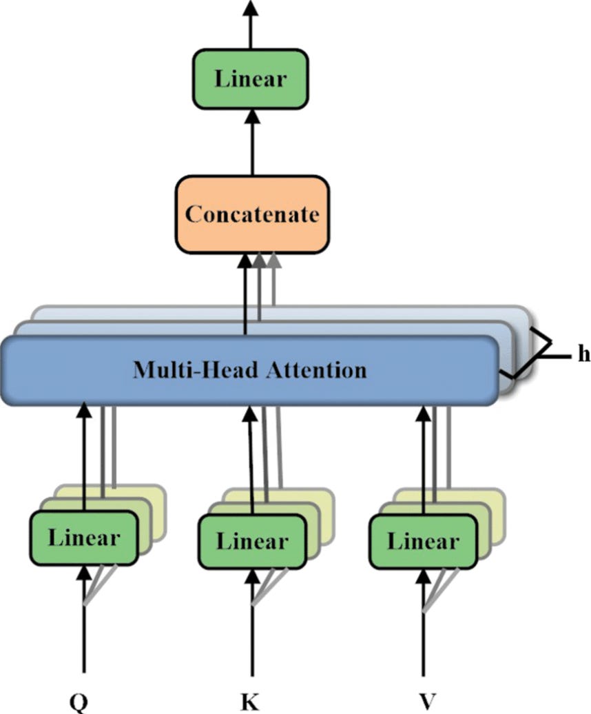
Each head uses its own Query, Key and Value weight matrix and produces head outputs that are concatenated.

\(\text{MultiHead}(X)=\text{Concat}(\text{head}_1,\dots,\text{head}_h)W^O\)

where,

\(\text{head}_i = \text{softmax}\!\big(\tfrac{Q_iK_i^\top}{\sqrt{d_k}}\big) V_i\)

Feed Forward Networks and Residual Connections

We introduce non-linearity by adding a feed forward network so that the model can pickup complex features.

\(\text{FFN}(x) = \text{ReLU}(xW_1 + b_1)W_2 + b_2\)

We also add residual connections and layer norm to stabilize the model and avoid Vanishing Gradients.

\(\text{output} = \text{LayerNorm}(\text{out}_1 + \text{FFN}(\text{out}_1))\)

With that, the Encoder block is complete.

Decoder

The Decoder is responsible for generating the output tokens. The contextual information that has been generated by the Encoder is used to generate outputs.
It does so using two inputs:
1. The tokens it has already generated.
2. Encoder’s contextual representation of the input sequence.

So, the decoder has to work with the tokens it has generated by itself to see what token would come next by looking at the input sequence that is important at that point in time.
Let’s look at this with the help of an example.

Input Sequence: ‘Kanishk is going to watch football.’

Decoder Output: ‘कनिष्क फुटबॉल देखने जा रहा है’ (A classic translation based transformer)

Let’s say the decoder has finished translating till the word ‘फुटबॉल’, then it will have to look at both the input sequence through the encoder output and the last outputs it has generated till now.

Hence, we use two Attention modules in the Decoder block.
They are:
Masked Multi-Head Attention
Cross Attention (Encoder Decoder Multi-Head Attention)

Masked Multi-Head Attention

Here, we need to ensure that the decoder can only see the tokens it has generated so far and not the tokens that are about to be generated (during training).
This is where masking and shift-right come into play.

Shift Right:
During training, the target sequence (the ground-truth output) is shifted one position to the right. This means we prepend a special token like [start token] to the sequence and move all other tokens one step forward.

\( \begin{array}{|c|c|} \hline \textbf{Decoder Input} & \textbf{Decoder Output} \\ \hline \texttt{[start token]} & I \\ I & love \\ love & cats \\ cats & \texttt{[end token]} \\ \hline \end{array} \)

This is done so that during training we create perfect pairs.

For example if we the start with the input ‘I’ itself without giving a start token, then the first token it generates would be ‘love’ and miss the token ‘I’.

Masking:
Even after shifting, we don’t want the decoder at position t to “peek” at tokens beyond itself. So we apply a causal mask (upper-triangular mask of -∞ in the attention scores) that blocks connections to future positions.

\(\text{Mask} = \begin{bmatrix} 0 & -\infty & -\infty & -\infty \\ 0 & 0 & -\infty & -\infty \\ 0 & 0 & 0 & -\infty \\ 0 & 0 & 0 & 0 \end{bmatrix}\)

This matrix is added to the score during Softmax so that the tokens can only see tokens before themselves.

For example:

For the sentence ‘I am a swimmer’, if we are at the word ‘a’ we hide the key/value vector of ‘swimmer’ from ‘a’ because ‘swimmer’ hasn’t been generated yet and to show the word ‘swimmer’ would affect the model learning and could be considered ‘cheating’.

Teacher Forcing:
At training time, instead of feeding the model its own previously generated predictions (which could drift if it makes mistakes), we feed the ground-truth shifted sequence as input.
For Example,
If the decoder doesn’t predict the word ‘love’ and predicts the word ‘hate’, we still pass the correct prediction ‘love’ as input to the Masked Attention module during training.
So that it doesn’t drift away due to the mistakes it can make during training.

Let’s unpack everything that happens in this block.

1. Each output token generated gets turned into Query, Key and Value vectors.

2. Same as in any attention module, Query compares itself with all Keys and gets a score.

3. Softmax turns these scores into weights.

4. We then add the masking matrix to the score to mask the values of the tokens that haven’t been generated yet.

5. So, the final attention score in this block is:

\(\text{Attention}(Q, K, V) = \text{softmax} \left( \frac{QK^\top}{\sqrt{d_k}} + M \right) V\)

This output is used to build a contextualized understanding of what has been generated so far by the decoder.

After this block, we add Residual Connections and Layer Norm and move onto the next Attention block.

Cross Attention

This attention module lets the decoder view the encoder’s outputs and act upon it.
Masked Attention focuses on what has been generated already, this one focuses on the encoder’s outputs and how they can be used to generate the next token.

The input Query tokens are the outputs from the Masked Attention block.
The Key/Value tokens used are from the Encoder outputs.

We compare the outputs from the Masked Attention block to see which part of input sequence should be attended to, while generating the next token.

Queries:

\(Q = H_{\text{decoder}} W^Q\)

Keys and Values:

\(K = H_{\text{encoder}} W^K, \quad V = H_{\text{encoder}} W^V\)

These keys and values act like a knowledge bank that the decoder looks up while generating the next token
Each decoder token’s Query compares itself against all of encoder’s keys:

\(\text{Score}_{ij} = \frac{Q_i K_j^\top}{\sqrt{d_k}}\)

This tells us which parts of the source sentence are relevant for generating this target token.
Let’s go back to the translation example.

Input Sequence: ‘Kanishk is going to watch football.’
Decoder Output: ‘कनिष्क फुटबॉल देखने जा रहा है
While the model is generating the next token say ‘देखने’, it would want to assign more importance to the word ‘watch’ as it corresponds to the next token.

So, the next token generation depends on both the previous token that has been generated- ‘फुटबॉल’ and the token from the input sequence that is most relevant - ‘watch’.

When generating the token “देखने”, the decoder’s hidden state (based on [start] कनिष्क फुटबॉल) is projected into a Query.

• This Query compares itself with the Keys of all encoder tokens (Kanishk, is, going, to, watch, football).

• The highest match occurs with the Key for “watch,” so its Value vector strongly influences the decoder’s next state.

• At the same time, the decoder also relies on its own self-attention (which already encoded “फुटबॉल”).

The model now has the contextualized understanding of the previously generated tokens and how they are related to the input sequence. This understanding is used to generate the next token.

We now add Residual connections and Layer Normalization the same as we do after any Attention block.

Prediction of tokens:

The actual prediction of tokens happens in this layer.
The decoder’s output is a sequence of contextual vectors.

\(\text{Decoder Output: } h \in \mathbb{R}^{T \times d_{\text{model}}}\)

We need to convert this into logits for every word in the vocabulary. (Probability of every word in the vocabulary being the next token)
We apply a linear layer:

\(Logits=h.W^t+b\)

For every token t you get a vector of size v representing it’s probability.

How prediction happens

The weight matrix here consists of the entire vocabulary of tokens

Each row represents a token

\(W \in \mathbb{R}^{V \times d} — \;the \;weight\; matrix\; in \;the\; final\; linear\; layer.\; \)

\(\mathbf{h}_t \in \mathbb{R}^{d} — \;the \;context \;vector \;from \;the \;decoder\;\)

Hence the dimensions match for every row in the weight vector to be compared to the entire context vector.

Note: In many models this output weight matrix is actually tied to the input embedding matrix so that the model has one shared representation space for both understanding words and generating them.

If the context vector matches a row (through the dot product) then it’s logit score would be high, so we look for how similar the context vector and each token row in the weight matrix is and assign logits according to that.

Each dot product tells us how aligned the context is with each word’s representation

A high dot product means that the current context vector is very similar to that word vector.

This linear layer essentially compares the context with every possible word in the vocabulary

We then use Softmax to get the probabilities:

\(P(y_t = w_i | \text{context}) = \frac{\exp(\text{logit}i)}{\sum{j=1}^{V} \exp(\text{logit}_j)}\)

The most probable token is the one whose embedding is most aligned (has highest dot product) with the current context.
This token is then generated.

That is how the Decoder generates the next token using the Encoder’s output and it’s own previously generated outputs.

Once the decoder generates the probability distribution for the next token, the model selects the most likely word and feeds it back to continue sequence generation. Repeating this process step-by-step allows the Transformer to produce coherent sentences, translations, or responses.

This was the working of the Transformer.

Conclusion

The Transformer laid the groundwork for all LLMs, but the landscape has evolved. Modern models rely on decoder-only architectures, mixture-of-experts layers, reinforcement learning, and other innovations. We’ll dive into these advances in upcoming blogs.

Thanks for reading, see you around soon!